The visualizer fills everything above the control bar. While Probe is playing it plots
the live signal pair in one of two modes, chosen with Mode; once you
freeze it shows the fitted
curve instead. Axes are unlabeled and fixed at full scale - both signals are clamped
to [-1, 1]. If no audio is arriving on the sidechain, Probe overlays a routing
reminder; how to route it
is covered in Capture and Save.
The transfer-function view
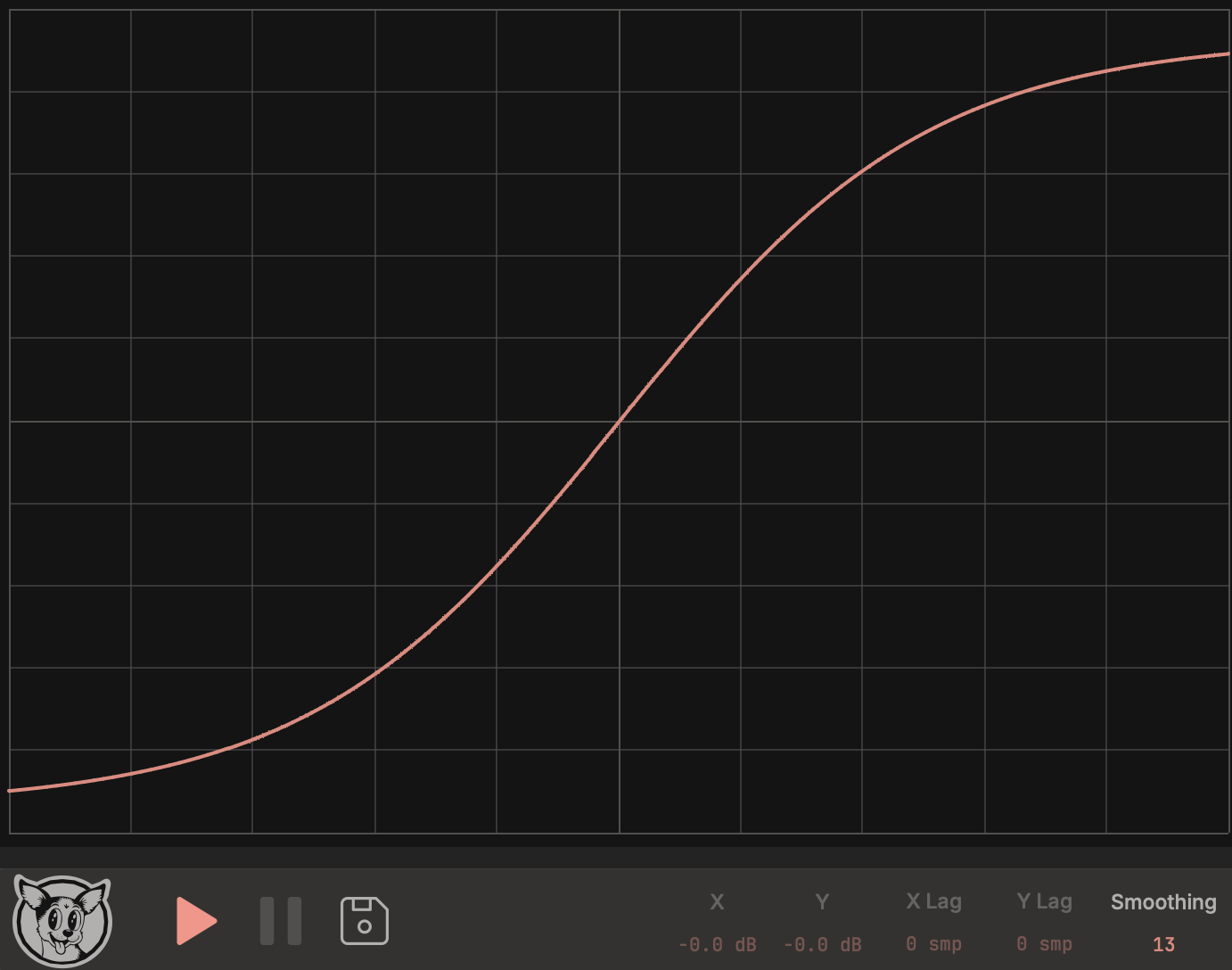
With Mode set to tfunc, the display is an XY oscilloscope of the two signals -
every sample lands at (input, output), so the device’s transfer behavior draws
itself in real time. The horizontal axis is the sidechain (the signal going into the
device under test); the vertical axis is the main input (the signal coming out of it).
A memoryless distortion traces a single clean curve. Time-dependent behavior - latency, hysteresis, EQ phase shift, anything where output depends on past input - shows up as a loop or smear. This is the same data the capture algorithm fits a curve to, so you can see whether a device is going to capture cleanly before committing. A loop that won’t collapse with latency compensation usually means real memory - see below.
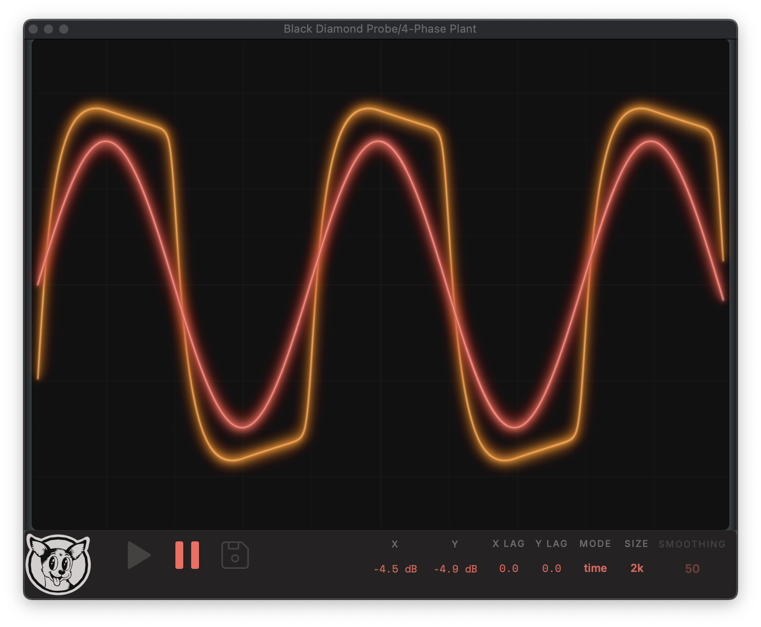
The time view
With Mode set to time, both signals are overlaid as waveforms on a shared axis -
the sidechain in front, the main input behind it. Size sets the visible window,
from 500 to 8k samples. The display triggers on a rising zero crossing of the
sidechain signal, so a periodic test tone holds still like it would on a scope. Useful
for matching levels, checking latency compensation, and seeing where in the waveform
the device is clipping or compressing.
Scale
The X and Y readouts show the visualization gain for each signal. Hover the readout to reveal the Scale X and Scale Y knobs, each from -36 dB to +36 dB. Scale only changes what you see - it is applied to the plot, not to the audio and not to the captured curve, so quiet signals can be made readable without touching your gain staging. Push a signal past full scale and the trace flat-tops against the display’s clamp; the clipping is only visual, but it hides detail, so back off if you see it. Scale is disabled while frozen.
Grid and draw options
Right-click the display to set Grid Strength (Faint, Medium, or Strong -
remembered between sessions) and Display Mode: Segments connects consecutive
samples with lines, while Scatter draws isolated dots, which reads better on spiky
or noisy signals where connecting lines would mislead. Display Mode resets to
Segments each time the editor opens.
What Probe can capture
For an accurate capture, the device under test must be memoryless - its output depends only on the current input, not on past inputs. Most distortion, saturation, and waveshaping circuits qualify. The catch is that they’re often packaged with DC blockers, EQ, or other tone shaping that introduces phase shift, which breaks memorylessness in practice. Bypass those if you can.
Devices with memory - compressors, EQ stages, anything with hysteresis (most tape saturation, magnetic circuits) - can still be interesting to visualize, but they can’t be reduced to a single transfer curve. The XY plot will form loops or drift over time, and any capture should be treated as a rough snapshot rather than a model.
Don’t write those captures off, though - even physics-based hysteresis models are built around a static transfer curve. The Jiles-Atherton model starts from the anhysteretic magnetization (saturation with the dynamics stripped out), then wraps it in nonlinear differential equations to add the feedback. Black Diamond Distortion’s Hysteresis mode lets you hijack that backbone - feed it any curve you’ve drawn or captured, and the physics rebuild the dynamics around it.